Transformations, Instancing, Multisampling and the Distribution Ray Tracing

This section includes the experiences of implementing object transformations, instancing, multisampling and distribution ray tracing. The depth of field, Glossy reflections (imperfect mirrors) and translation motion blur is added to our ray tracing model.

1. Transformations

Input

So, for new features new elements come to the input XML file. Transformations are given under the attribute same name. It can be scaling, translation or rotation. The first two ones are only 3D vectors, but rotation includes angle in degree and rotation vector as 3D vector, respectively. Any kind of object can be transformed via list under this attribute. These transformations are applied in the given order.

<Scene>
    <Transformations>
        <Translation id="1">0 -6 0</Translation>
        <Scaling id="1">3 0.1 0.1</Scaling>
        <Rotation id="2">0 0 1 0</Rotation>
    </Transformations>

    <Objects>
        <Mesh id="1">
            <Transformations>r1</Transformations>
        </Mesh>
        <Triangle id="1">
            <Transformations>s1</Transformations>
        </Triangle>
    </Objects>
</Scene>

Code Design

I have used GLM library for all transformation and vector-matrix multiplications. Until this section, I have used my own vec3 class and its methods. Thus, I renewed the code pretty much by replacing all vectors.

Transformations are added to the Scene class as a list of string where the first character indicates the type of transformation and the remaining number is the identification number of the transformation. In order to speed the process, all matrix multiplications are done in preprocess and saved as a localMatrix and inverseLocalMatrix element to the Object class.

Algorithm

When implementing transformation, I transformed the ray by the inverse transformation matrix of the current object instead of transforming the objects. In other words, coming rays are firstly inversely transformed and then processed in the intersection tests of objects (explained in the previous sections).

In my first approach, I planned to use the same things for Bounding Boxes. But, in preprocessing, bounding boxes are combined to a new bounding box. Thus, they had to be in the same space to be added properly. Because of this reason, I could not apply the same methods for bounding boxes. In preprocessing, bounding boxes were created from the points of transformed objects and then, in intersection tests, the world ray was directly tested with them. Let’s see its effects in the following part, implementation process, and why I changed my approach :)

Class Object
function intersect(ray, origin):
1. ray <- inverseLocalMatrix * ray;
2. origin = inverseLocalMatrix * origin;
3. apply remaining (in the previous part) intersection tests

Implementation Process

Firstly, I planned to generate the following scene.

Of course, not everything was as easy as described above :D When I thought that I was doing everything perfectly as described above, I got the following result (left image).

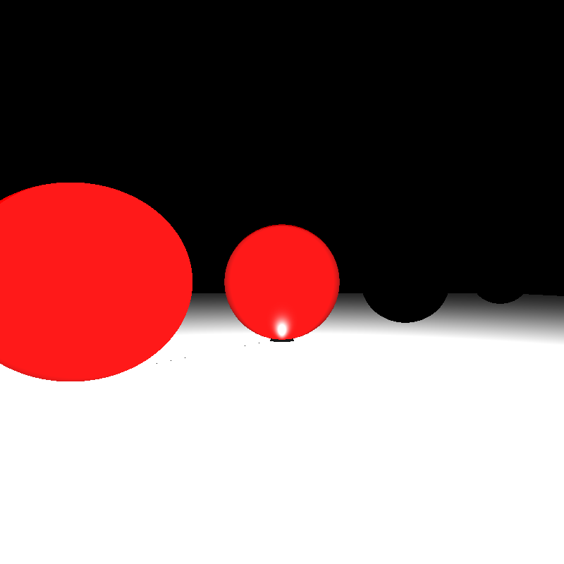
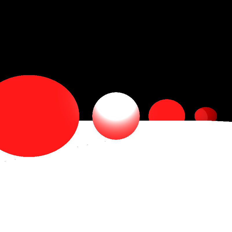
I realized that I forgot to normalize ray directions after these transformations. After that I got the result above (right). Now, the problem seemed to be related to shading because light directions didn’t look correct and the scene was too bright. I checked the shading function and realized that all shading operations were done via non-transformed ray. In addition, after a ray comes from the intersection test, if it is intersected with an object, the ray should be inversely transformed again for remaining shading operations. After fixing these, the result would be below (left).

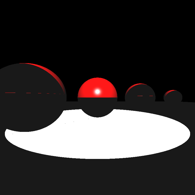
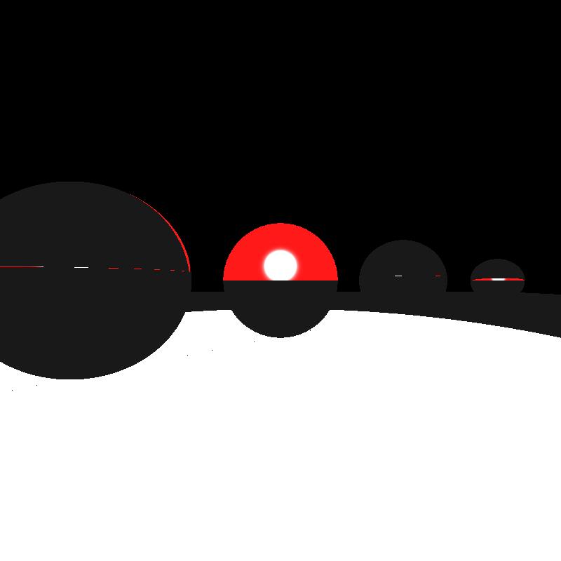
It is clearly seen that the spotlight was not in the correct direction because I needed to transform the light direction to the inverse local space of the object, as well. After fixing related operations on the shading function, I got the result in the above figure (right). But, there were some problems still. Shadows didn’t look correct. Yes, I had to re-transform intersection ray (with localMatrix of the object) to be sure that it would be ready to intersect with other objects for shadow testing. The result can be seen in the following figure (left).

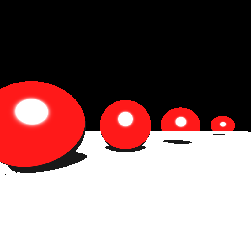
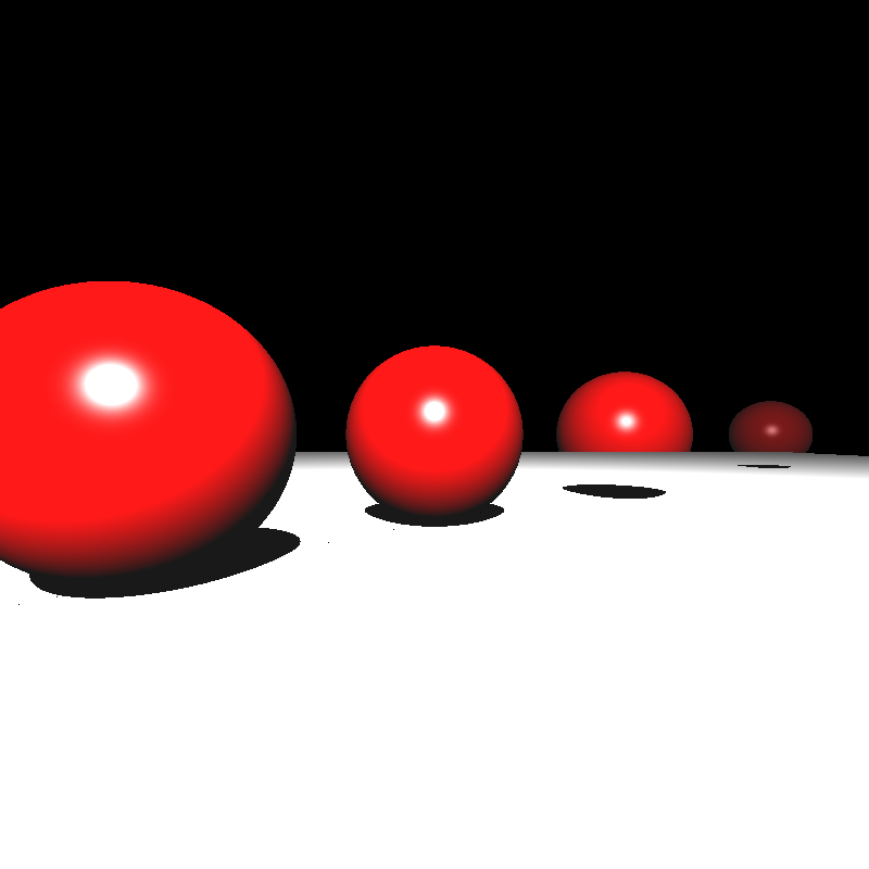
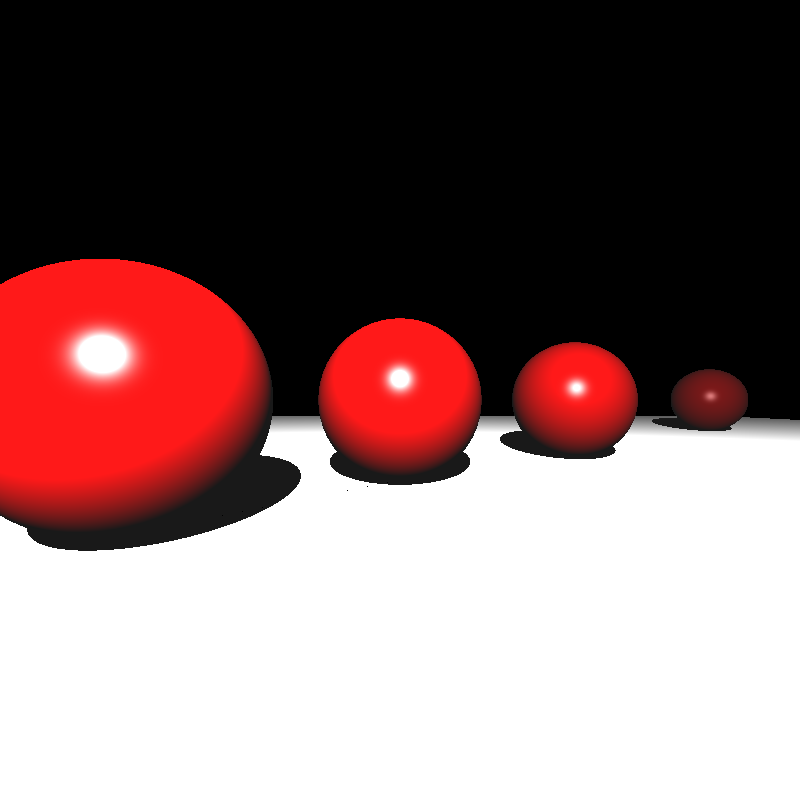
The intensity was divided by the correct distance between light source and hit point (in shading function). In addition, obviously, mesh normal vectors had some problems. After fixing the calculation of normal vectors, I got the correctly transformed result in the below.

Ok.. But this approach was so painful and wasteful! I realized that instead of transforming everything with the inverse transformation matrix, I can just transform the normal vector of objects :D It is more easy to implement and absolutely more faster by avoiding many operations. I switched this method and got the same results.

2. Instancing

Input

For the instancing part, instances are defined using the element. These objects are copied from the base mesh object with the given additional feature below.

<Scene>
    <MeshInstance id="5" baseMeshId="1" resetTransform="true">
        <Material>3</Material>
        <Transformations>r1 t3</Transformations>
    </MeshInstance>
</Scene>

Code Design

I added a new class for mesh instances. In proprecessing, a new mesh object is created for each mesh instance. Its transformation matrix is generated according to the resetTransform element.

Algorithm

I used the same vertex data for mesh instances by pointing them. By this way, we can prevent wasting redundant memory. After creating a new mesh object in preprocess, everything will be the same for ray tracing.

Implementation Process

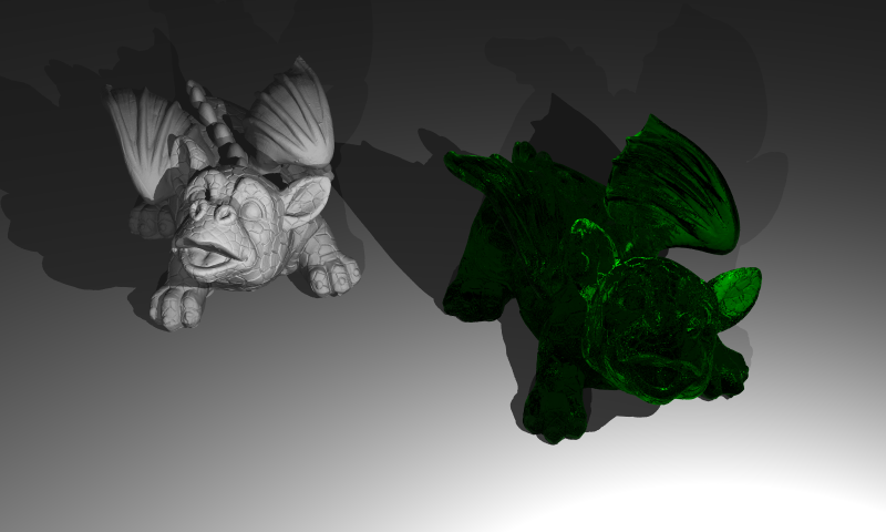
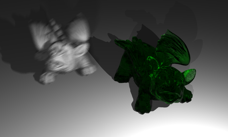
Below we can see the very first result of implementation of the mesh instances. The right green dragon will be generated by using the same vertices of the left dragon. Its transformation matrix and material are just different from the base mesh.

Note that models have some sprinkles. This effect will be improved by implementing the multisampling in the next part.

3. Multisampling

Input

The third part, Multisampling is enabled by adding the field to the Camera element.

<Scene>
    <NumSamples>N</NumSamples>
</Scene>

Algorithm

With this feature, multiple small random samples for each pixel will be generated and filtered. I have used the average filter for final pixel color.

function createScene():
1. for each camera
2.     initialize camera
3.     for each pixel
4.         color <- initialize
5.         for each sample
6.             generate random number inside the pixel
7.             compute ray direction by adding randomness
8.             color <- color + rayTracer(ray)
9.         color <- color / numberOfSamples
10.    write color information to the image file

Implementation Process

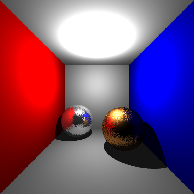
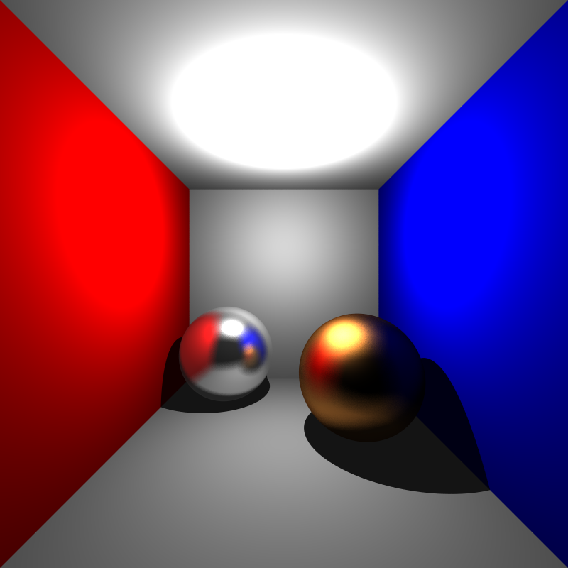
Multisampling gets more smooth edges as seen in the example image below. Left images show the before multisampling effect. It is straightforward and I did not use any difficulties during its implementation.

4. Distribution Ray Tracing

Input

The final part of this section is the Distribution Ray Tracing. This includes various visual effects with very little extra cost over multisampling. These effects are depth of field, glossy reflections and motion blur. Required elements for this part are given below.

<Scene>
    <FocusDistance>21</FocusDistance>
    <ApertureSize>1.5</ApertureSize>
    <MeshInstance id="1" baseMeshId="7" resetTransform="true">
        <MotionBlur>0 0 4</MotionBlur>
    </MeshInstance>
    <Material id="4" type="conductor">
        <Roughness>0.1</Roughness>
    </Material>    
</Scene>

The field of and will be used for the depth of field. We assume that there is a flat square lens on the aperture. Glossy reflections refer to imperfect mirrors. This is indicated by the presence of the element in the material attribute. will be used for the blurry appearance of fast moving objects. It is assumed to be only for translational movements. The element defines a final translation of the object during which the image capture was taking place.

Algorithms

Depth of Field

Real cameras have finite aperture as opposed to the pinhole model we have been using so far. Without a proper lens, a finite aperture camera is guaranteed to produce blurry images on its image plane. A lens is a glass contraption which allows focusing objects at a certain distance from it to a single point behind the lens. This is known as the focal or focus distance of the lens. Photographers typically put their main subject at this distance to create an effect where the subject is sharp but the background is blurry. In distributed ray tracing we can simulate this effect to make our renderings as if they are coming from a real camera (are taken from the notes of Assoc. Prof. Dr. Ahmet Oğuz Akyüz)

Figure-1: Depth of Field

function createScene():
1. for each camera
2.     initialize camera
3.     for each pixel
4.         color <- initialize
5.         for each sample
6.             generate random number inside the pixel
7.             ray.dir <- compute ray direction by adding randomness
8.             generate random values between [-0.5,0.5]
9.             dx, dy <- scale the random values to camera.apertureSize
10.            s <- camera.u*dx + camera.v*dy + camera.position;
11.            t <- camera.focusDistance / dot(ray.dir, -camera.w);
12.            p <- ray.dir*t + camera.pos as a ray.origin;
13.            ray.dir <- normalize(p - s);
14.            color <- color + rayTracer(ray)
15.        color <- color / numberOfSamples
16.   write color information to the image file

Glossy reflections

This effect is generally used to simulate metallic objects that are not polished. Brushed metal is an example. It allows a reflection ray to be sent at an angle that is somewhat off from the perfect reflection direction. This effect again involves randomness (are taken from the notes of Assoc. Prof. Dr. Ahmet Oğuz Akyüz).

function reflectionRay(ray, normal, roughness):
1. ray.dir <- compute reflection ray direction as previous sections
2. ray_prime <- ray.dir.copy()
3. axis <- argmin(abs(ray.dir))
4. ray_prime.axis <- 1
5. u <- normalize(cross(ray.dir, normalize(ray_prime.dir)))
6. v <- cross(ray.dir, u)
7. n1, n2 <- generate two random values between [-0.5,0.5]
8. ray.dir = normalize(ray.dir + roughness*(n1*u + n2*v))

Motion Blur

We can compute the Motion Blur effect by generating multiple rays in different times [0-1]. These ray times are generated initially and do not change while reflecting or refracting. Time 0 and 1 represent the initial and final positions of the object, respectively. A translation of a ray at any time in this interval is interpolated according to the motion vector. Note that this translation is independent from our transformation matrices in the previous part.

Only intersection tests of objects and bounding boxes are affected from motion blur as given below. I multiplied the origin of ray with the translation matrix of motion. Because we assumed that motion is done only by translation, ray direction cannot be changed by multiplying any translation matrix.

 function intersect(ray, origin, rayTime):
 1. m <- compute translation matrix at rayTime by motionBlur vector
 2. m <- get inverse of m
 3. ray.origin <- m * ray.origin
 4. do intersection test with the ray

Implementation Process

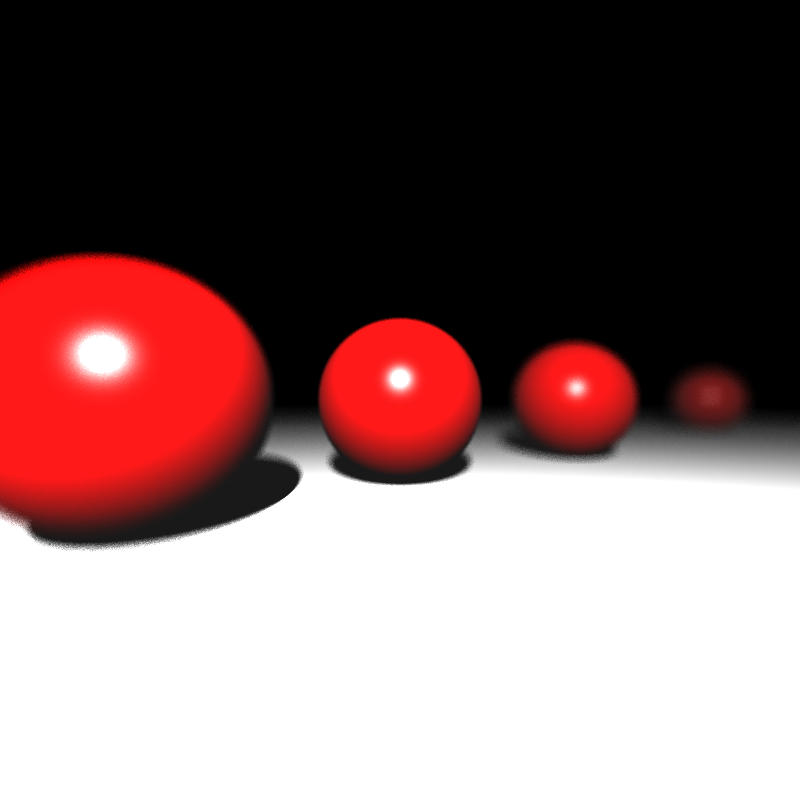
The before and after result of the Depth of Field effect can be seen below. But, there was a problem with the focusing area.

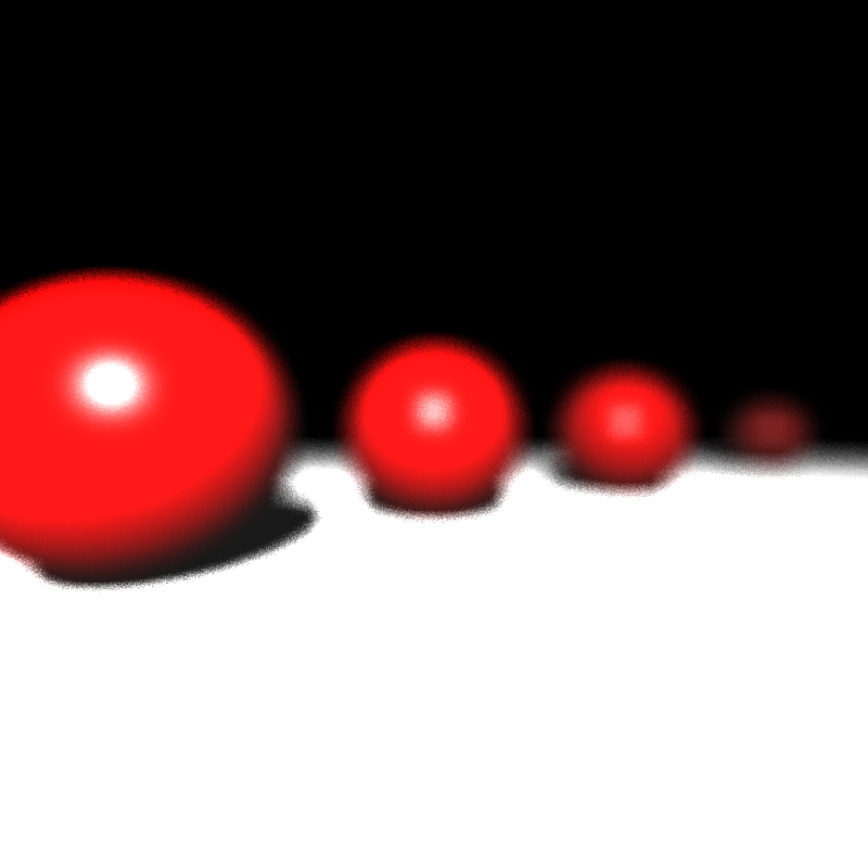
After spending many hours, I realized that the origin of my primary rays was the camera position instead of the point of s (given in Figure 1). Final before and after result can be seen below.

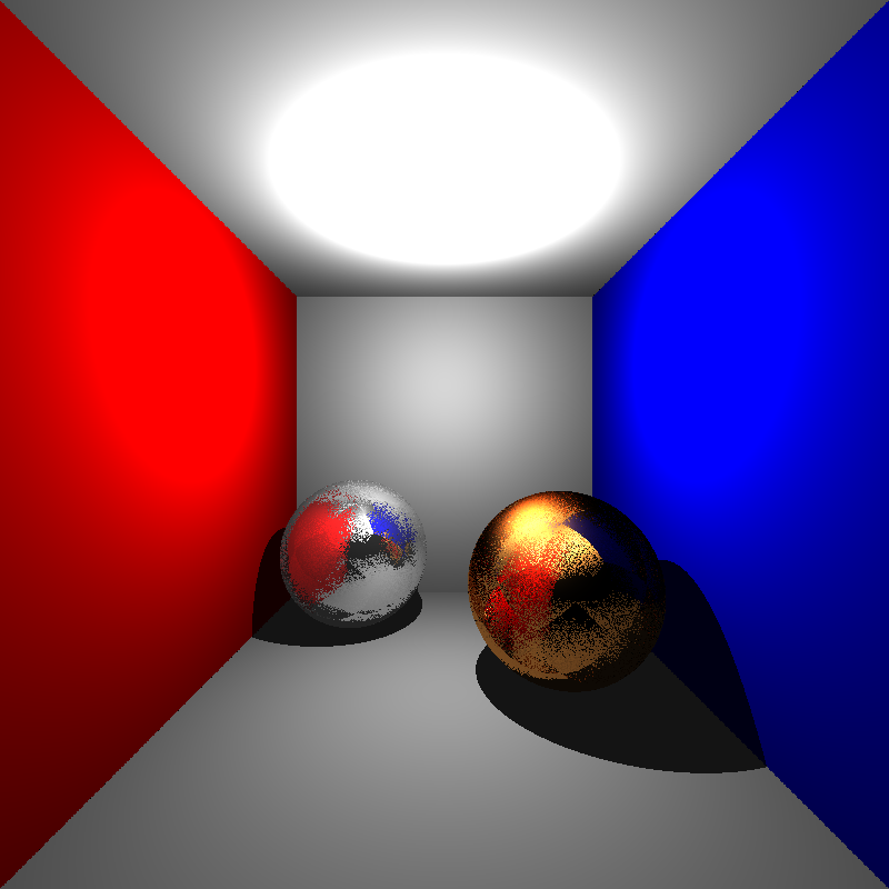
The very first result of the Glossy Reflection is given below. Obviously, something was wrong on the left. Thanks to Alper Sahistan, I realized that my normalized random number n1 and n2 should be between -0.5 and 0.5 instead of 0 and 1. After fixing it, I got the true result on the right.

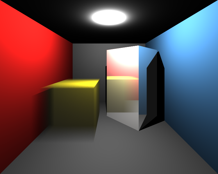
Let’s see the result of motion blur. We want to move object from left image to the right image.

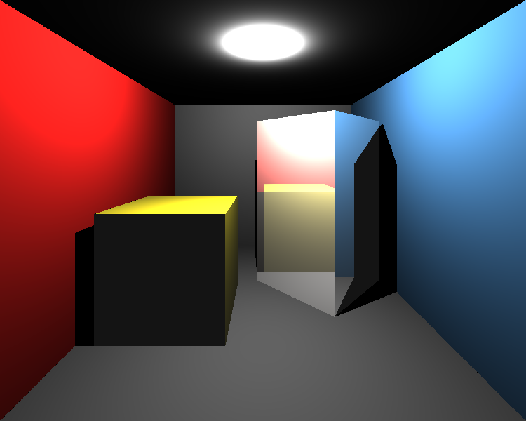
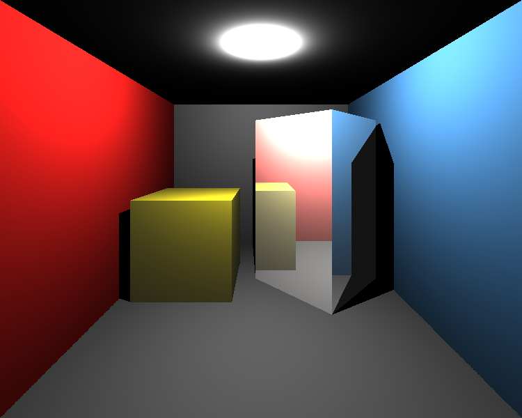
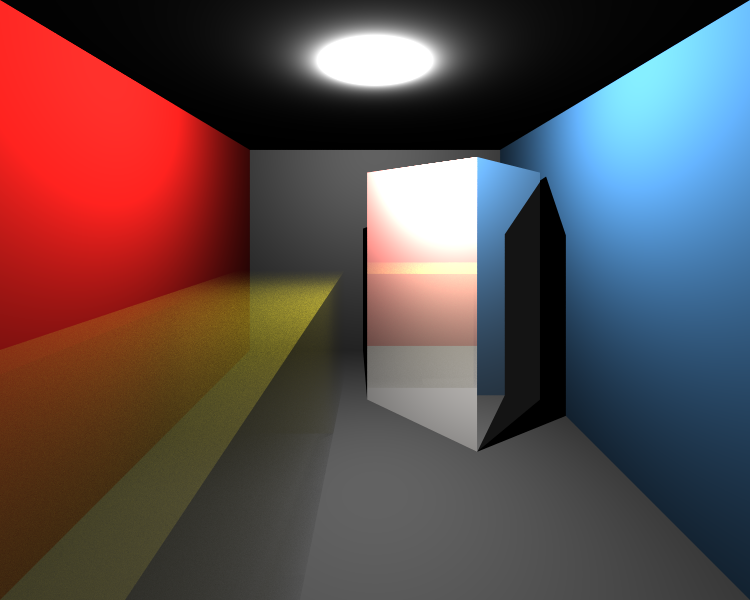
Firstly, I was confused about the order of transformation multiplications in the intersection tests. I mean that I could not decide to multiply ray with the inverse motion translation or inverse object transformations matrices. I tried the multiply ray with inverse motion translation matrix after transforming it to the object local world. But, as seen below (left), it was wrong for the given motion vector. Its effect would be too much if it is applied at non-local space. After changing the order I got the true result as seen right images.

Other Improvements

Bugs on Dielectric Materials

As we know from the previous section, when an incident ray intersects with a dielectric object, it produces two rays: refraction and reflection ray. I assumed that the refraction ray is always inside (i.e. its color is suffered from absorption) and the reflection ray is always outside (i.e. its color never is suffered from absorption). But it was an absolutely wrong assumption.

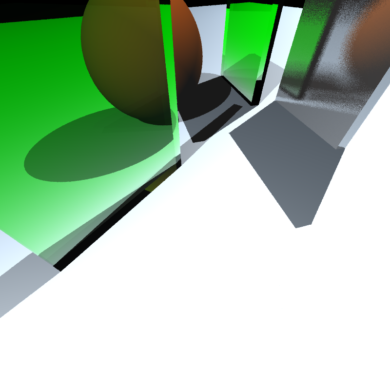
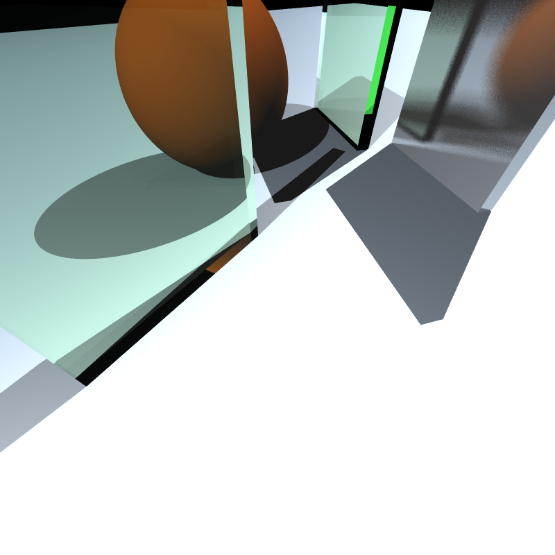
If an incident ray is already inside (i.e. refraction ray of another ray) its generated reflection ray will be inside, as well. Thus, we have to apply absorption to this ray instead of the generated refraction ray. It solves the problem seen in the left image.

Surprisingly, this mistake didn’t have any effect on previous dielectric scenes, so I could not be aware of that until now.

Time Improvement

The running times of almost all of the examples were larger than I expected because many of them have huge numbers of Multisampling. Creating a single scene takes less than a second in many cases, but creating the same scene with 500 times more takes linearly increasing time. With my pure BVH implementation, most of the scene took 10-15 minutes. Just generating one sample from dragon_dynamic.xml took around 2 hours, and the scene is composed of 100 samples. I need to improve the BVH.

For this purpose, instead of combining the boxes of different objects, the root node can be divided into main objects (not faces). Thus, we do not need to transform vertices to compute the combining bounding box. By this approach, if a ray intersected with the bounding box of a mesh, it will be transformed with the inverse transformation matrix of an object one time. Then, all intersection tests of faces of the object will be in its local space. Therefore, there is no need for any more transformation.

This approach made BVH more than 100 times faster so generating all 100 samples of dragon_dynamic.xml takes around 75 mins instead of 200 hours!

Final Results

Let’s look at the final results of my implementation after all improving.

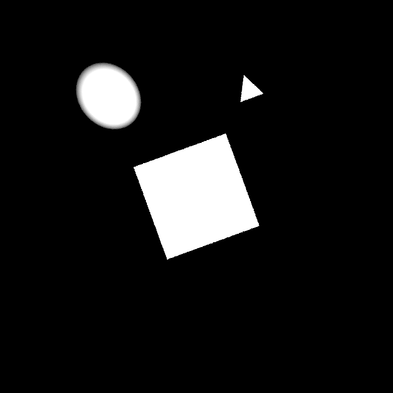
simple_transform.xml

XML file is parsed in 0 sec
Maximum BVH depth is 1
Preprocessing is finished in 0 sec
Scene is created in 0 sec

spheres_dof.xml

XML file is parsed in 0 sec
Maximum BVH depth is 1
Preprocessing is finished in 0 sec
Scene is created in 38 sec

cornellbox_boxes_dynamic.xml

XML file is parsed in 0 sec
Maximum BVH depth is 2
Preprocessing is finished in 0 sec
Scene is created in 390 sec

cornellbox_brushed_metal.xml

XML file is parsed in 0 sec
Maximum BVH depth is 1
Preprocessing is finished in 0 sec
Scene is created in 214 sec

metal_glass_plates.xml

XML file is parsed in 0 sec
Maximum BVH depth is 2
Preprocessing is finished in 0 sec
Scene is created in 87 sec

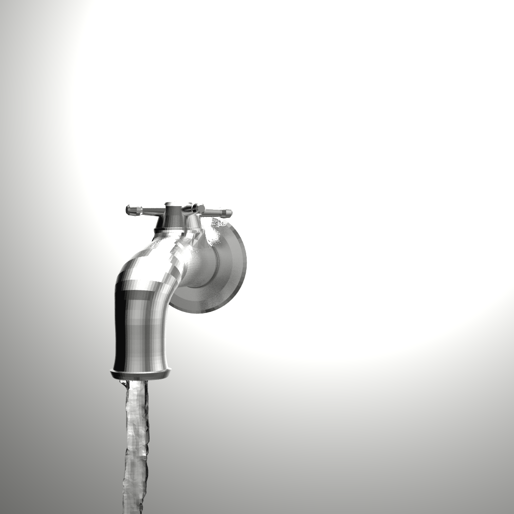
tap_0200.xml

XML file is parsed in 0 sec
Maximum BVH depth is 17
Preprocessing is finished in 0 sec
Scene is created in 333 sec

dragon_dynamic.xml

XML file is parsed in 6 sec
Maximum BVH depth is 19
Preprocessing is finished in 10 sec
Scene is created in 4352 sec

eksuas.github.io

Transformations, Instancing, Multisampling and the Distribution Ray Tracing

1. Transformations

Input

Code Design

Algorithm

Implementation Process

2. Instancing

Input

Code Design

Algorithm

Implementation Process

3. Multisampling

Input

Algorithm

Implementation Process

4. Distribution Ray Tracing

Input

Algorithms

Depth of Field

Glossy reflections

Motion Blur

Implementation Process

Other Improvements

Bugs on Dielectric Materials

Time Improvement

Final Results

simple_transform.xml

spheres_dof.xml

cornellbox_boxes_dynamic.xml

cornellbox_brushed_metal.xml

metal_glass_plates.xml

tap_0200.xml

dragon_dynamic.xml